 GaⅤin.com by Gavin W.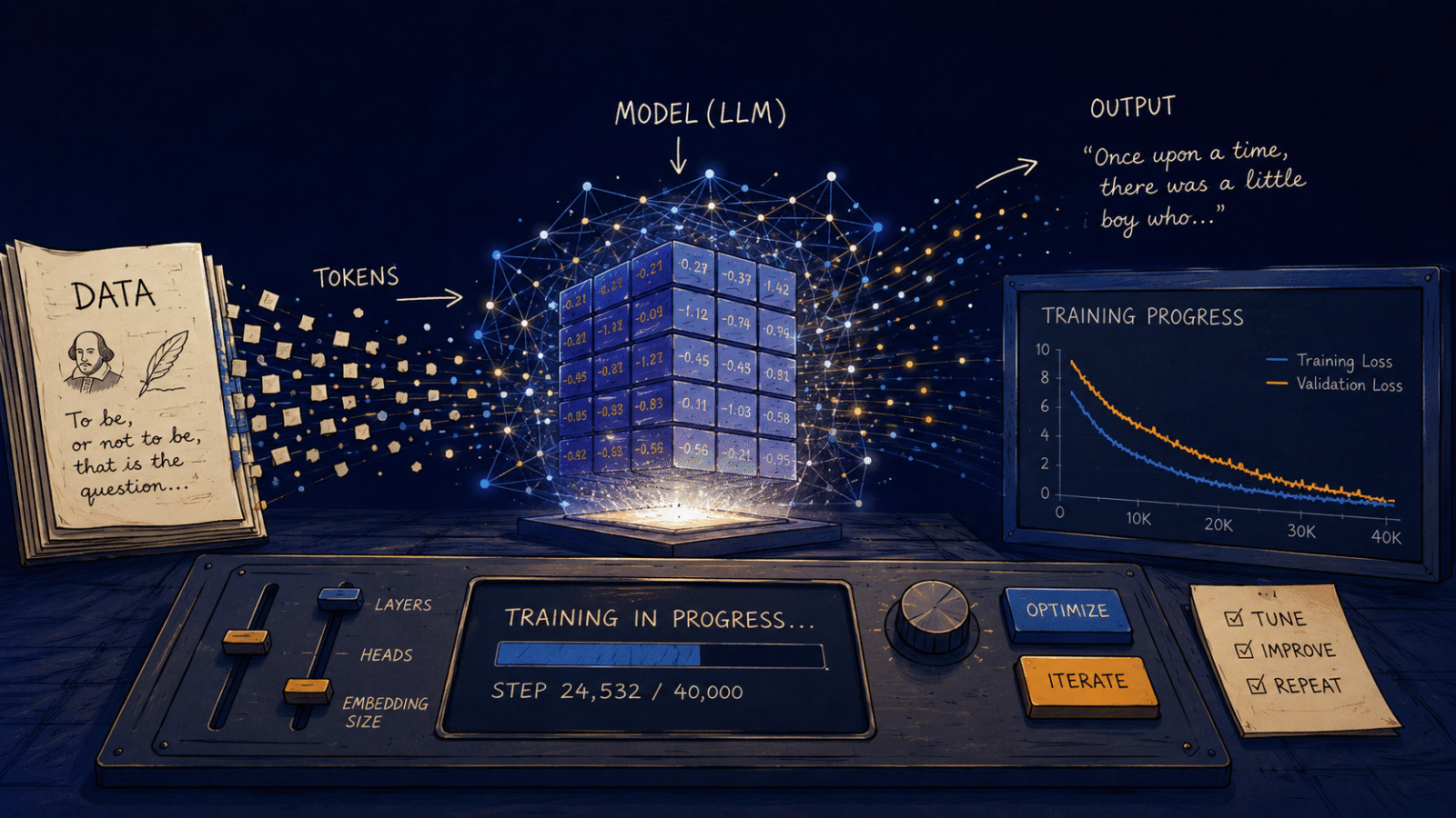
Training an LLM can seem like a dark art. The realm of trillion dollar companies working away in massive datacenters. But that’s not always the case. It’s totally possible to train a simple LLM on your own hardware, and it’s a great way to learn about how they work.
This is built on LLM From Scratch, which walks you through building a tiny LLM trained on Shakespeare’s works. After seeing how easy and fast it can be to run it, I added a few extra bits to make it faster, and output clear charts during the training process. I’ve made the code needed for this more acessible on GitHub.
This turns out to be an excellent way to learn about the basics of LLM training, and see some of the problems that can arise. The lessons can also apply to other forms of machine learning, prediction errors are not unique to LLMs!
Setup
Tiny stories is a dataset of short stories that I found on the web. By keeping the language to only a small set of words that a 5 year old could understand, it makes the dataset small enough to train on my RTX 5060 Ti relatively quickly, and still be complete English. It is available on HuggingFace. The specific set I used is his V2 set. I used two versions, the full 2 GB set (542 Million tokens) and a smaller 20 MB set (4.5 Million tokens), to show what can happen with too small datasets.
For the tokenizer, I used a simple BPE based approach with 8192 tokens. One of my early mistakes was trying only 256 tokens. It turns out that the tokenizer always reserves the first 256 tokens for the English character set. Unless you are making a custom tokenizer focusing on character level LLMs, you will need a larger token set.
The Charts
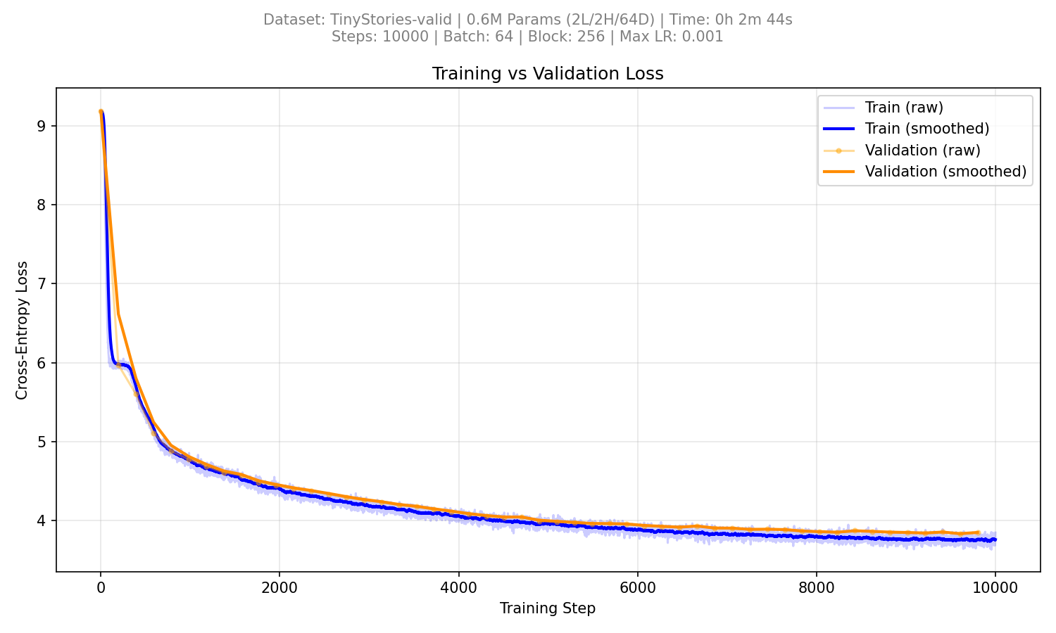
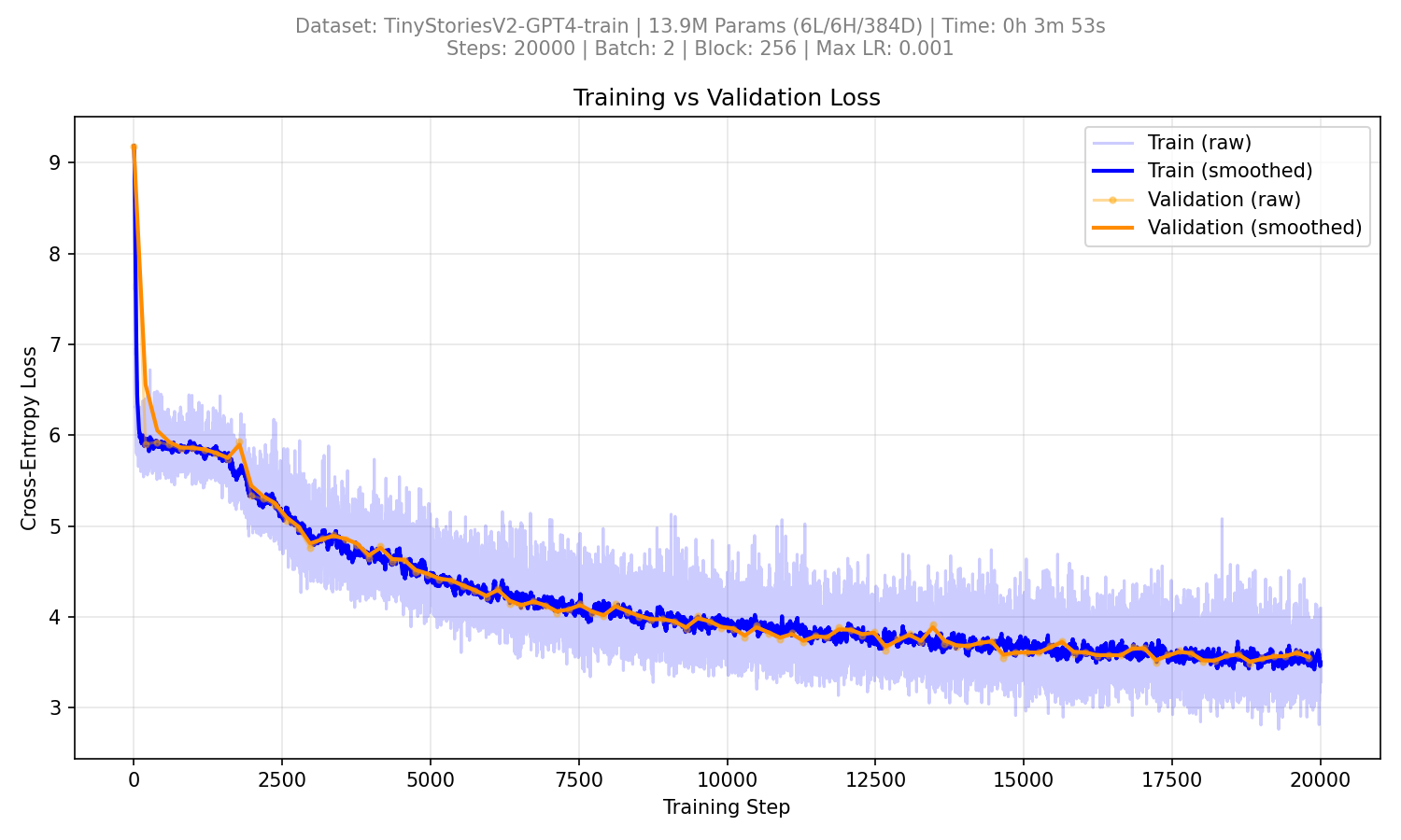
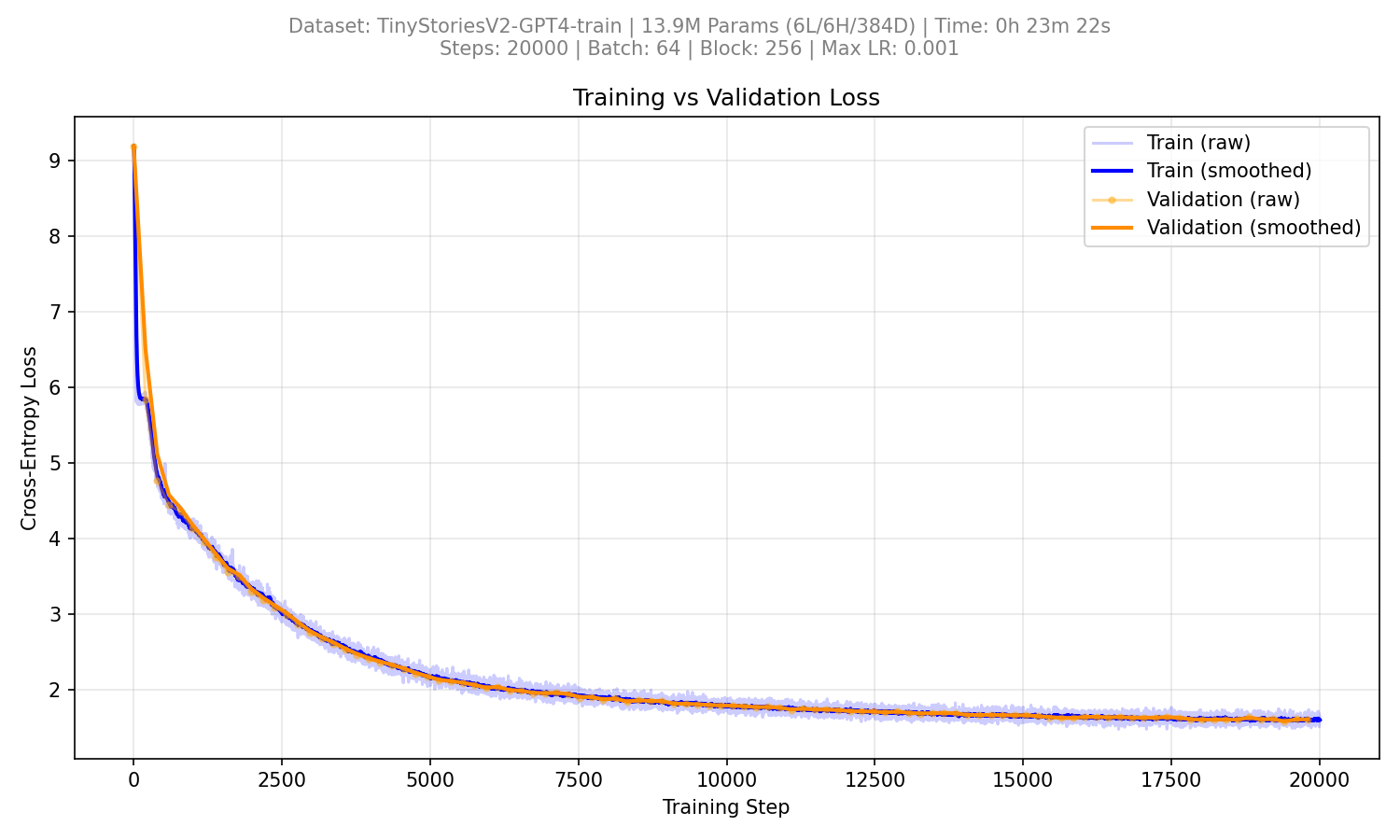
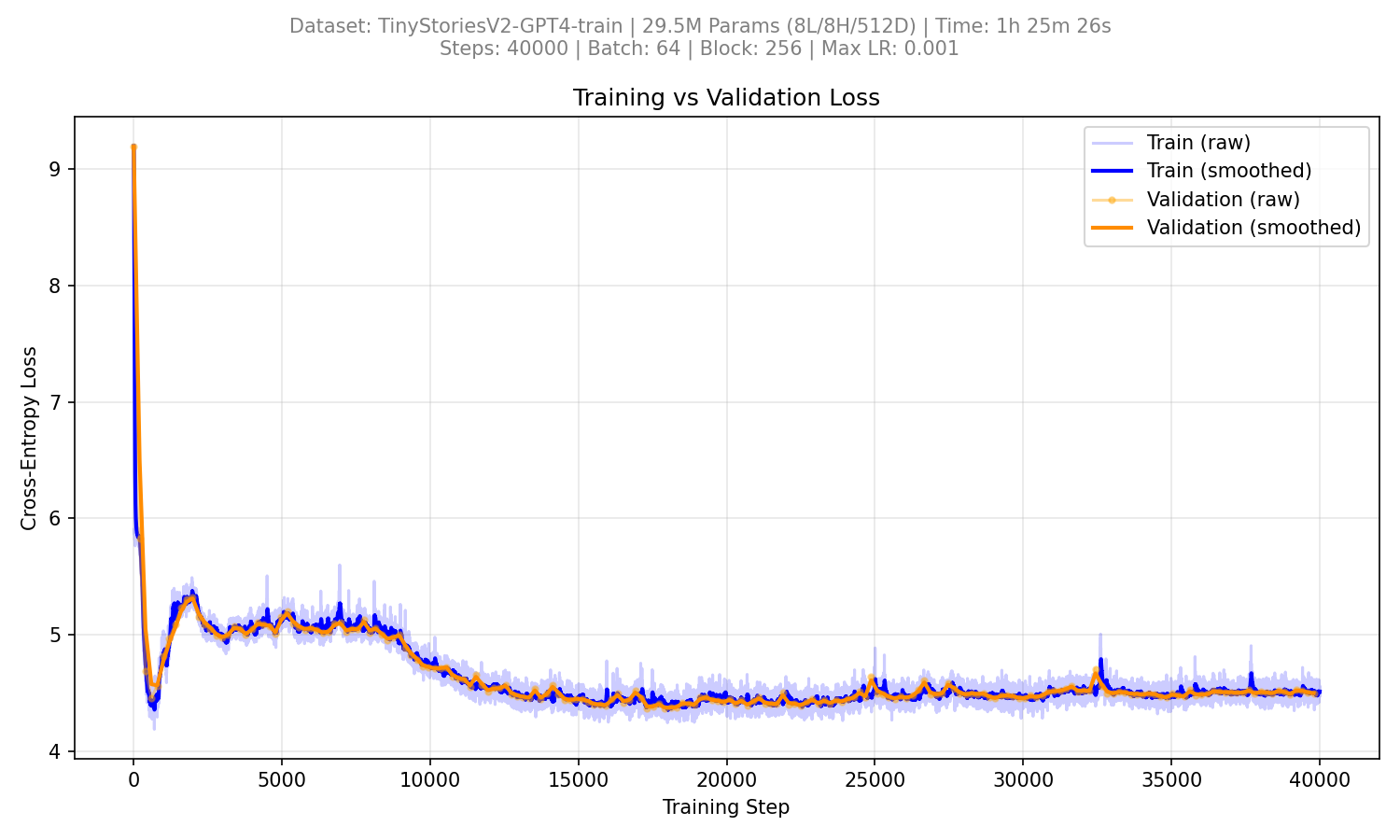
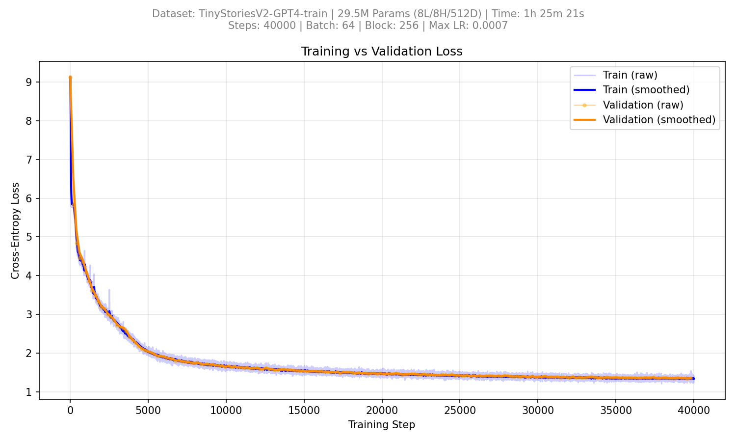
The included charts show the relationship between training loss and validation loss during model training. Training loss (blue line) is essentially how well the model is matching data during the training run, so how well it’s learning the training data. Validation loss (yellow line) is how well the model is matching data it’s never seen before, so how well it can generalize to new data. Over time we want to see both of these trend downwards and match each other. Values near 9 mean that the model is guessing randomly, while values closer to 0 means it’s doing a good job of predicting the next token.
How big is your brain?
One of the first things to decide when making an LLM is how big the transformer architecture will be. Major commercial LLMs have billions to trillions of parameters, but for our toy one, we can get away with just a few million.
The number of parameters essentially sets the overall intelligence of the model. How much it can remember and how well it can reason. It’s a bit more complicated than that, but it’s a good rule of thumb. It’s made up a few tunable parameters.
The n_layer is the number of transformer blocks. It’s how “deep” the model can reason and remember patterns. One layer may focus on adjacent words, while the 4th layer may focus on sentence structure, and the 8th on the overall story.
The n_embd is the size of the embeddings. This is the size of the vectors that are used to represent the tokens. The larger the number, the more information can be stored in each token. The higher this value the more meaning the model can fit into each individual word.
The n_head is the number of attention heads. This is the number of different ‘views’ the model has of the input sequence. It allows the model to focus on different parts of the input sequence at the same time, or how the individual words relate to the others.
It’s best to keep these balanced with each other. For example, if you had 2 layers and 1024 embd it would have a rich vocabulary but limited reasoning (shallow and wide), while 12 layers and 128 embd would have a deep reasoning capability but limited vocabulary (deep and narrow). Additionally, the number of attention heads and layers must be a divisor of the embedding size.
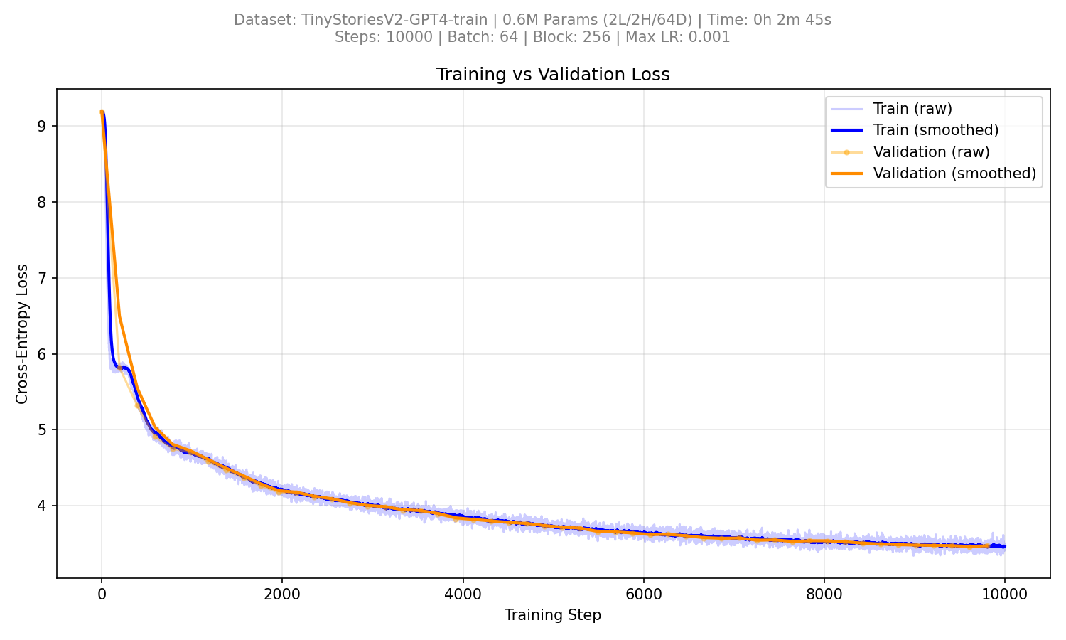
These first charts show what happens when the model is too small for the dataset. I set Layer and Head to 2, and embed to 64 (0.6M parameters).Both the larger dataset and the smaller dataset stop at about 4 loss. They get to a certain point, and then they just stop improving.
Sample Output:
Once upon a time, there was a time there was a special friends lived around his friends. He loved and she wanted to play with her backyard. One day to sing. One day, Sarah loved to go outside and decided to have a little girl was so sad.
Adding more data doesn’t help as the model is just too small. The only option here is to go to a bigger model.
Sample Output:
Once upon a time, there named Tim, a little girl named Tim was a walk. But then, he found a big red cat. Tim said, “Hi, Sam, I’m a moment and said, “Yes, do not help me? You are my home. She had to play the bird, “I can I love you want to play.” Ben. You have a moment and have so happy. It was so she got inside his friends playing in the tree.
Overfitting Data
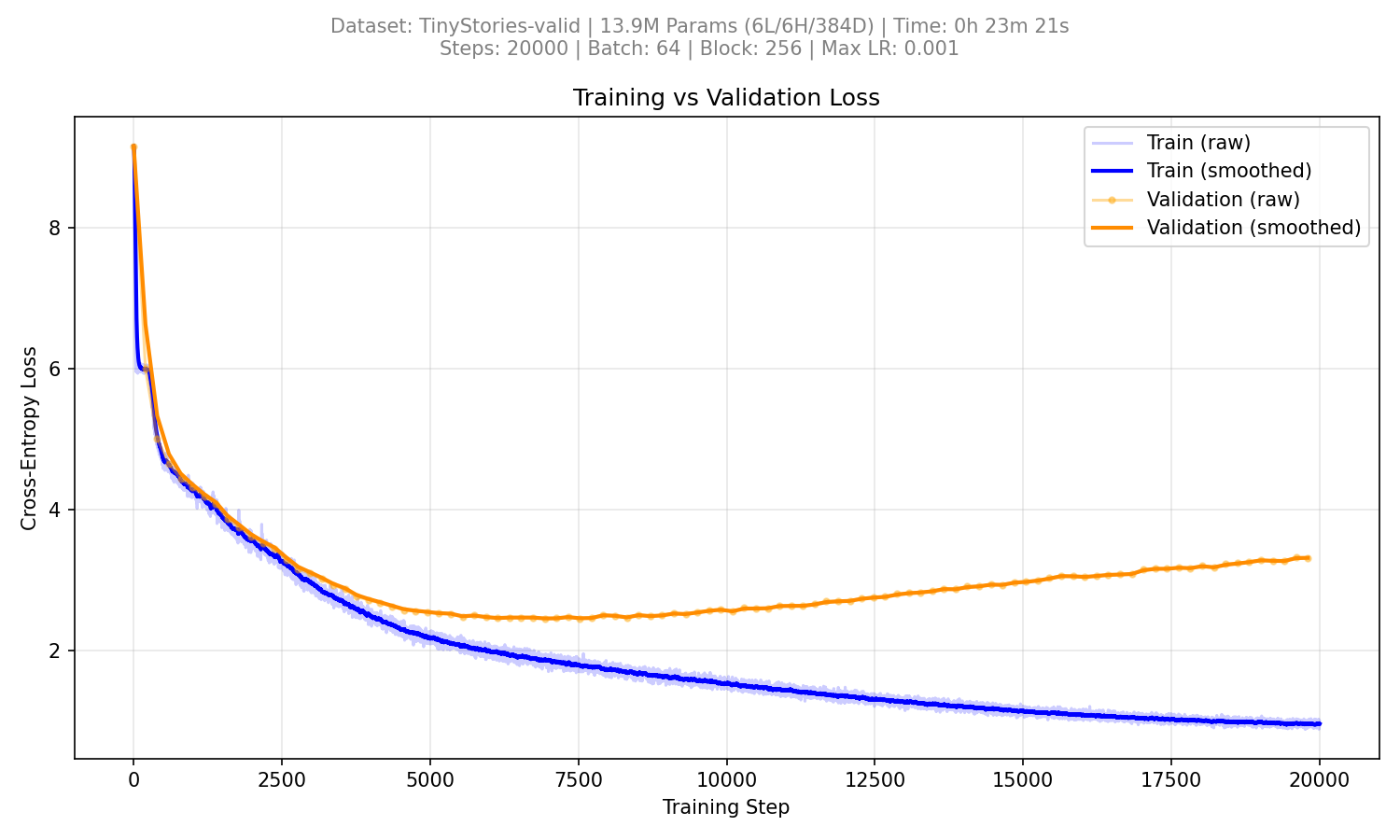
So let’s try a larger model. 6 layers, 6 heads, and 384 embd (13.9M parameters). Trying to train a model of this size on only 4.5M tokens is a recipe for disaster, as you can see from the chart. It quickly memorizes the training data, but can’t generalize to new data. This is represented by the validation loss line shooting up as while the training loss continues to drop.
Sample Output:
Once upon a time, there was a little boy named Tim. Tim liked to play with his toys all day. One day, Tim found a big, red ball in his room. It was so big that he could fit in his room. “Ouch!” cried Tim. his mom came into the room, saw the ball and got a big, angry truck. “Uh oh Tim!” Tim wanted to help Tim. He was a dependable boy. He asked his mom if he could repair the truck for now. His mom said yes, and together they put the truck back together. When Tim and his mom returned home, Sue felt proud of himself. She knew that organizing things was important and that they could fix anything. From that day on, Tim
Batch Sizes and Random Data
Another tunable aspect of the training process is the batch size. This is the number of tokens that are processed at once before it makes a change to the model weights. It’s a balance between the speed of training and the quality of the training. Smaller batch sizes train faster, but introduce randomness into the model. This causes the model to sporadically pingpong back and forth during training as minor variance in the training data has a greater effect on the model. For this run we use a batch size of 2 instead of 64. In this chart it shows as the wide changes in the raw training loss data and irregular validation loss.
Sample Output:
Once upon a time, there was a beautiful frog. Tim was so he loved to the world to have a picture. He thought the park and made it and his things. The little boy took them. They made a toy and laughed, and had lots of the sun with the best. They did not so they were the cat had lost all lived happily together. They saw a big truck had many friend.
Let’s give the model a fair chance to show what it’s capable of. We’ll use the larger 542M token dataset with a batch size of 64. We see a smooth training line, and validation loss decreasing steadily and uniformly.
Sample Output:
Once upon a time, there was a little boy named Tim. He liked to play outside in the sun. One day, while playing, he saw a mysterious tree in his yard. He wanted to climb it, so he tried to climb the tree. As Tim climbed, he saw a beautiful view. He saw many birds and animals playing. Tim felt very happy and wanted to join them, so he started to climb the tree. As Tim climbed higher, he met a girl named Sue. Sue saw the unknown view and said, “Wow! That is a new thing to do!” She smiled and said, “Thank you, Tim! I will be here to help you.” And from that day on, Tim and Sue would always build a happy tree
Pretty decent output, but there’s more we can get out of the dataset if we go larger…
LLM Cram School
Another tunable parameter is the learning rate. This is the amount that the model weights are adjusted during each step of the training. It’s a balance between the speed of training and the quality of the training. Smaller learning rates train slower, but introduce less randomness into the model. This causes the model to sporadically go off the rails during training as minor variance in the training data has an outsized effect on the model. It can somewhat be offset by using a larger batch size, but to a certain extent large models need more time to learn the patterns.
We have been using a learning rate of 1e-3 (0.001). This is a relatively high rate, but it was working fine before. But trying the same settings on a larger 8 layer, 8 head, 512 embed model causes some issues. Notice how the loss drops, then starts to rise again. The optimizer got off track by trying to change too much too fast and could never recover.
Sample Output:
Once upon a time, he. The bird.The day, a little girl went to play and went was the big park of said to get the hill. One day, Max saw him the big red bird. She was a little box, to to the girl. They took a lot. The big day was she and the friend. The the cat came and very the park. He went. Everyone was aTom saw a friend to to saw the sky and her friends. The were he, the ground and the big tree was the new bird the. The dog, fast because Tom. The very proud. He was so surprised. The saw a excited, the little wind! box. They loved around was her tree with the ground with a and her big
This 2nd chart isn’t quite as random, but shows the loss falling, then rising again as the optimizer goes off on a tangent - it eventually recovers, but the damage is done.
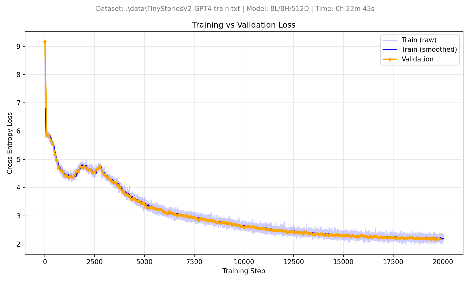
Let’s drop the learning rate by even a small amount to 7e-4 (0.0007). There’s some small instability, but overall the model is learning much better, and we finally get good looking output!
Sample Output:
Once upon a time, in a small town, there was a boy named Tom. Tom had a big dog named Max. They liked to play catch with a ball. Tom would throw the ball, and Max would run to get it. They were best friends. One day, Tom and Max went to the park to play. They saw a new girl named Sue. Sue was very shy and did not talk much. Tom and Max decided to play a game to see who was the best. Sue was very good at the game and made many friends. Tom and Max played the new game every day. They had lots of fun together. Sue was not shy anymore. Tom and Max learned that it was better to play together and have fun. And they lived
Areas to Imporve
This is a simple starting point. We’re only tuning a few basic paramaters. We use a simple cosine decaying learning rate schedule, but there are others to consider. One quick improvement would be watching the validation loss and stopping training when it stops decreasing, or starts to increase. This would stop you from wasting GPU time trying to improve a model that isn’t going to learn anything more. A more complex option would be to implement a dynamic learning rate scheduler that adjusts the learning rate based on the validation loss. THere’s a built in ReduceLROnPlateau scheduler that does exactly this.
Conclusion
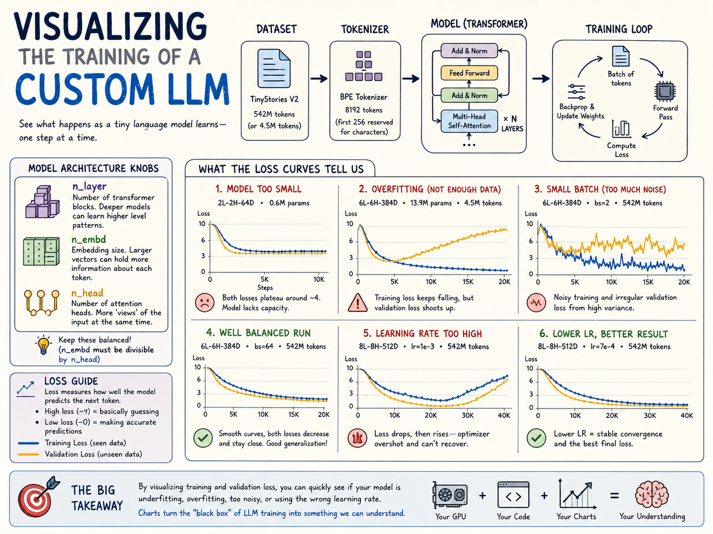
Training an LLM doesn’t have to be a mystery locked away in enterprise datacenters. By scaling down the dataset and tweaking the transformer dimensions, anyone with a modern GPU can experiment with these models. Tuning parameters like the number of layers, embedding dimensions, batch size, and learning rate is a delicate balancing act—but visualizing the training and validation loss curves makes it much easier to spot when the model is underfitting, overfitting, or simply crashing due to an overly aggressive learning rate.
While our simple model won’t be passing the bar exam anytime soon, building one from scratch provides a foundational understanding of how tools like ChatGPT actually learn to write.